Layer-Wise Relevance Propagation

TL;DR

Layer-Wise Relevance Propagation (LRP) is a propagation method that produces relevances for a given input with regard to a target output. Technically, the computation happens using a single back-propagation pass, similarly to deconvolution. I propose to illustrate this method on an Alpha-Zero network trained to play Othello.

Table of content

• LRP Framework
  • Formulation
  • Different Rules for Different Layers
  • Technical Details
• Interpreting Othello Zero
  • Playing Othello
  • Network Decomposition
  • Interpretation
  • Evaluate an Explanation
• Resources

# LRP Framework

Formulation

LRP @1 is a local interpretability method which attributes relevance to any neuron activation inside a neural network with regard to a target output and a given input. The target output can be non-terminal (e.g. an intermediate layer neuron activation), multi-dimensional (e.g. the final vector of logits) or uni-dimensional (e.g. a single class logit). Its formulation is similar to the classical Gradient$\times$Input @2 as it is computed using a single modified backward pass. Yet, it doesn’t suffer from the noisiness of the gradient.

Notation

The activation of the $j$-th neuron in the layer $l$ is noted $a_j^{[l]}$ and its associated relevance is noted $R_j^{[l]}$ and by convention $a_j^{[0]}$ represents the input and $R_j^{[L]}$ the target output. Weights are indexed similarly such that if the layer $l+1$ is linear its weights are noted $w_{kj}^{[l+1]}$ (torch convention) and $b_k^{[l+1]}$ performing the mapping, to the $k$-th neuron of the layer $l+1$, given by equation $\ref{eq:linear_mapping}$ where $g$ is the activation function.

Figure 1 illustrates the process of relevance propagation, which can be intuited as a redistribution flow. The relevance $R_k^{[l+1]}$ is decomposed in “messages” sent to the previous layer. The message, $R_{j\leftarrow k}^{[l\leftarrow l+1]}$, from the $j$-th neuron of the layer $l+1$ to the $i$-th layer of the layer $l$ is then given by the equation $\ref{eq:message_decomposition}$, where $\Omega_{jk}^{[l+1]}$ is the decomposition rule (see bellow). The new relevance $R_j^{[l]}$ is then obtained by summing each “message” sent, as described by equation $\ref{eq:message_aggregation}$.

Decomposition Rules

A rule $\Omega_{jk}^{[l+1]}$ defines how to redistribute the relevance $R_k^{[l+1]}$ of the layer $l+1$ into the previous layer $l$. The ideal rule depends on the nature of the layer $l+1$ and is an active topic of research @3@4@5 (e.g. for new or more complex architecture like Transformers), more on this in the rule and evaluation sections.

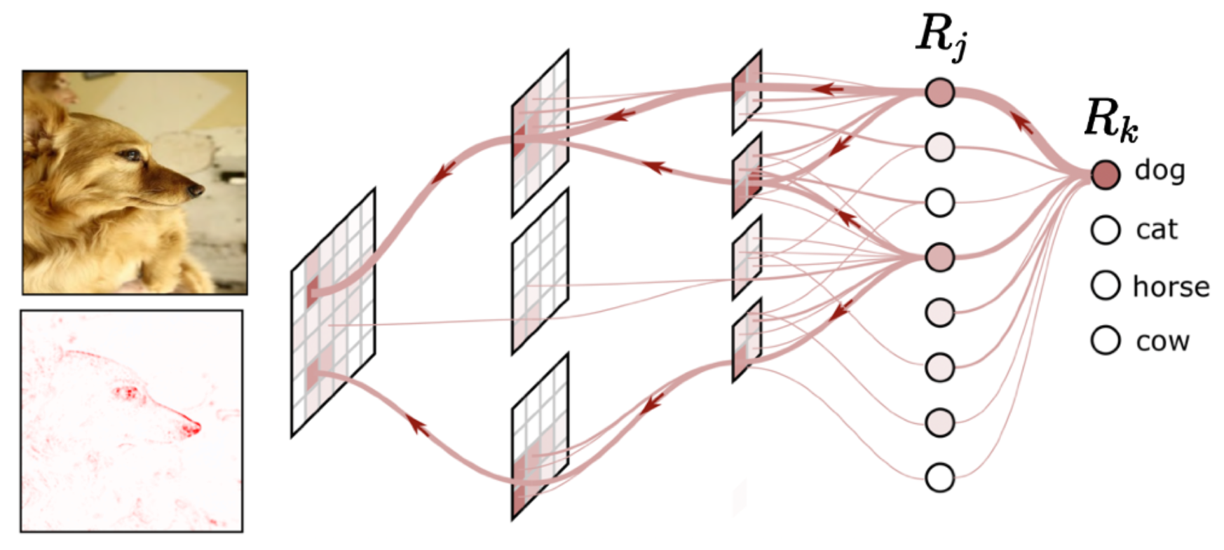Figure 1: Relevance back-propagation of the dog logit, @5.

The most basic LRP rule @1 is given by the equation $\ref{eq:original_lrp_rule}$, which is a simple pre-activation weighting. One drawback of this rule is that it is not conservative, i.e. $\sum_jR_{j}^{[l]}\neq\sum_kR_{k}^{[l+1]}$ $\Leftrightarrow$ $\sum_j\Omega_{jk}^{[l+1]}\neq1$, and thus relevance get lost or created by the bias along the propagation. Therefore, this rule was revisited by @5 as LRP-$0$ by setting the biases to $0$ (a trick).

Generalisation Gotcha

The layer superscript is sometimes omitted in the literature because it doesn’t cover the general formulation. For example, to account for residual connections, the propagation should be spread across multiple layers. The general formulation is thus simply given by a causally weighted sum $R_{j}=\sum_{k}\Omega_{jk}R_k$ where the numbering is across all the neurons (causally means $\Omega_{jk}=0$ if $k<=j$, messages are only sent backwards). It is less informative about the practical implementation but still carries the idea of tracking the actual computation.

Different Rules for Different Layers

Intuitively, the relevance propagation rules should be dependent on the layer’s nature, as is the forward flow. Fundamentally, this idea comes from the ambition of tracking the model’s various kinds of actual computation into each relevance. The classical framework for deriving these rules is Deep Taylor’s series Decomposition (DTD) @6, yet it should be justified with care @7. I’ll now present the necessary rules needed for the experiments I conducted, whose derivation can be found in the various linked resources (most of them assume ReLU, which is the case here).

Notation

The layer superscript is dropped in this section for readability and since all the rules will be applied on consecutive layers. The index $j$ still refers to layer $l$ and the index $k$ to layer $l+1$.

LRP-$\epsilon$ @1: Defined by the equation $\ref{eq:lrpe_rule}$, it introduces $\epsilon$, a numerical stabilizer and the $z$ coefficients are set accordingly to the equation $\ref{eq:original_lrp_rule}$ ($z_{jk}=w_{kj}a_j$ and $z_k=\sum_{j}w_{kj}a_{j}+b_k$). A variant of this rule can be computed by setting the biases to $0$, but this is not enough for the propagation to be conservative. The stabiliser $\epsilon$ will absorb some relevance and should, therefore, be kept as small as possible. In practice, this rule is made for linear mappings (Linear & BatchNorm).

$z^+$ @6: Defined by the equation $\ref{eq:zplus_rule}$, where $w_{kj}^+$ stands for the positive part of $w_{kj}$, i.e. $w_{kj}^+$ if $w_{kj}<0$. This rule is conservative and positive (and thus consistent @6). In practice, this rule is used for convolution.

$w^2$ @4: Defined by the equation $\ref{eq:wsquare_rule}$, this rule is meant for early layers. This rule is conservative and positive (and thus consistent). In practice, it is used for the first layer, e.g. in order to propagate relevance to dead input neurons.

Flat @4: Defined by the equation $\ref{eq:flat_rule}$, this rule is similar to $w^2$ but assuming a constant weighting. It, therefore, redistributes equally the relevance across every preceding neuron. This rule is conservative and positive (and thus consistent). In practice, it is used for the first layer, e.g. in order to propagate relevance to dead input neurons.

Technical Details

All the LRP computation can be done using the original authors’ library Zennit @8. In practice, the graph and back-propagation mechanism of torch.autograd is used using backward hooks; see the snippet below. The models need to implement the forward pass only using proper modules (child of the model instance) for them to be detected by Zennit and hooked. And since it relies on full back-propagation, every module of the graph should be hooked (even activation functions).

Pass rule: This is a practical rule necessary regarding Zennit implementation. In practice, even activation functions should be hooked because otherwise, the classical gradient will be computed during the backward pass. And since the actual relevance propagation is carried by other module hooks (Linear, Conv, etc.), no modification should be done (it’s a pass-through). It is typically used for activation functions.

This important snippet explains how backward hooks are coded in Zennit, which is fundamental to designing new rules. Besides Rules, derived from the BasicHook, other fundamental objects are available:

• Stabilizers: $\epsilon$ term in the LRP-$\epsilon$, which make the computation numerically stable. All rules are used in practice.
• Canonizer: Needed when using BatchNorm layers @3, to reorder the computation.
• Composites: To easily combine rules.

To illustrate rules, below is a snippet of the $z^+$ rule implementation. The first element is param_modifiers, which is used to modify the weights of the module, like here to separate positive and negative weights or like in LRP-$0$ to set the biases to zero. Then there are the input_modifiers and the output_modifiers, which enable lightweight modification of the forward pass (using the modified weights). In the rule below, they are used to separate positive from negative inputs. Finally, the gradient_mapper is used to compute the final form of the rule ($\Omega_{jk}$) here, one for positive and one for negative contribution, and the reducer computes the module relevance ($R_j$).

# Interpreting Othello Zero

Playing Othello

Before digging into the actual interpretation of the network I borrowed from Alpha Zero General @9, it is important to understand how it is used in practice and how it was trained. I highly recommend checking their code on Github or the associated blog post as well as the original Alpha Zero paper @10.

Tree representation of game (Min-Max, Alpha-Beta, MCTS, …) is an intuitive representation of a game whose main components are the root (the current position), the nodes (board states $s$) and the edges (action chosen for a given state $(s,a)$). Regarding search, the Alpha Zero paper @10 used MCTS PUCT @11, with the upper bound confidence (UCB) given by the equation $\ref{eq:upper_confidence_boundary}$. This equation involves network predictions (heuristic) with $P_\theta(s)$ the policy vector and $Q_s$ is the average expected value over the visited children (terminal reward or intermediate network evaluation, i.e. the value $v_\theta(s)$). $c_{\rm puct}$ is a constant to balance exploitation with exploration and after multiple rollouts the action is often chosen according to the tempered visit distribution, $\pi_s$ , given by the equation $\ref{eq:visit_distribution}$, with $\tau$ the temperature.

The network is trained by combining the loss from the value and the policy predictions. It especially makes sense since these predictions share a common graph (architecture) in the model. The value output $v_\theta(s)$ should predict the ending reward of the game $z$ (-1, 0 or 1 depending on the outcome) and the policy output $P_\theta(s)$ should predict the action sampling distribution obtained after search $\pi_s$. The loss is then @10:

In my drafty accompanying notebook , I chose functional version of this algorithm, with few minor changes from the Alpha Zero General code. Also, I put below a slightly modified version of the MCTS that is compatible with the LRP framework. The idea is quite simple: you have to keep track of the gradient in order to perform a backward pass under Zennit context later. In this way, you could interpret the aggregated quantities $Q_s$ and $U_s$ in terms of relevance. These quantities carry information about the subsequent tree from node $s$ and could be used a posteriori or during inference.

Disclaimer

This last piece of work is only exploratory, and I have made no digging in this direction yet. However, I am convinced that refining and experimenting in this direction could lead to interesting tracks like tree analysis or relevance-guided search.

Network Decomposition

In order to use Zennit, it is important to remember how it is implemented and adapt the network accordingly. First, all used modules should be instantiated under the target module (even activations). Then softmax should not be used because of the exponential. Here, it can be safely removed as the output is the Soflogmax, which is a simple translation of the raw logits and doesn’t change the action sampling.

The network architecture is quite simple as it is a basic CNN mostly using ReLU activation. For the convolution layer, I’ll use the $z^+$ rule, and for the linear mapping (including batch normalisation), I’ll use LRP-$\epsilon$. These settings are recommended, but you could try various different ones. To evaluate the different combinations of rules, refer to the evaluation section.

Gotcha

It is important to acknowledge the similarity in computation for the value and the policy. This will expectedly lead to very close relevance heatmaps as only one layer differs between the two.

One practical limitation for interpreting board games concerns the empty cells. Using traditional LRP rules will attribute zero relevance to those cells. Indeed, during the computation, the model doesn’t use these pixels but rather uses biases. In order to overcome this difficulty, I propose to use the Flat or the $w^2$ rules in the first layer.

Interpretation

Disclaimer

The following experiments are highly shallow, and I don’t pretend they are highly relevant or valuable. This work is only for illustrative purposes and definitely needs more digging. If you are interested in a follow-up of this project (by yourself or by me) and/or have questions, feel free to contact me.

I’ll now study a particular board picked during a self-played game with different parameters for black and white ($c_{\rm puct}=0.1$. for black and $c_{\rm puct}=2$ for white) using 10 rollouts per move and keeping the data from the previous moves. Playing multiple games with these parameters shows that the middle game is dominated by black while the endgame is dominated by black, i.e. exploration is a long-run payoff. I picked board 31 (black to move) as it is balanced (before black domination). Using the described rules, with Flat in the first layer, the relevance heatmap obtained is plotted in Figure 2. The value relevance is localised around the best move (B6), found by the MCTS, and negative or close to 0 around illegal moves.

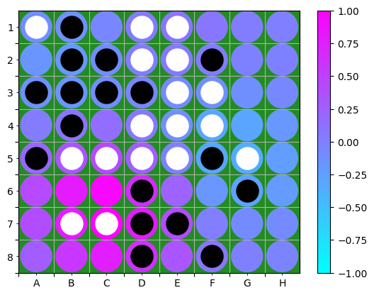Figure 2: Value relevance heatmap using Flat, $z^+$ and LRP-$\epsilon$, normalised by the maximum relevance amplitude.

Yet, is it really what I think it is? Remember that the biases and the Flat rule are used here to compute the relevance. With the same rules, using an empty board yields the heatmap of Figure 3.

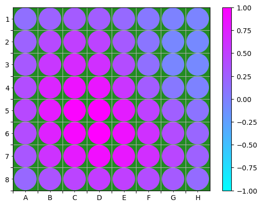Figure 3: Value relevance heatmap of the empty board using Flat, $z^+$ and LRP-$\epsilon$, normalised by the maximum relevance amplitude.

If it is harder to interpret, I’ll leave it for a more comprehensive study and change the Flat rule for a $z^+$ rule (the first layer is a convolution). This then yields the value relevance in Figure [4] and the policy relevance in Figure [5]. The value relevance is still localised around the best move, but it might be a correlation. Indeed, the relevance seems to indicate that the networks attribute more value to the pieces flipped by the move A7 that put a piece on the side. The way the network perceives value in sides and corners should be dug more. The policy relevance heatmap is more difficult to interpret, and note that the sign is due to logit initialisation. Yet, it attributes more relevance to the pieces flipped by the move B6.

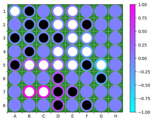Figure 4: Value relevance heatmap using $z^+$ and LRP-$\epsilon$, normalised by the maximum relevance amplitude.

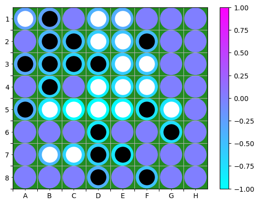Figure 5: Policy relevance heatmap using $z^+$ and LRP-$\epsilon$, normalised by the maximum relevance amplitude.

The next section describes how to evaluate the explanation’s faithfulness and robustness. Yet it was not successful as the board games add an extra layer of complexity since the input space is sparse. More complex considerations are needed.

Evaluate an Explanation

It is important to keep in mind that producing a heatmap is easy, but interpreting it in a faithful way is much harder. What’s more, you also have to be careful about what actually is what you are visualising. There is sometimes a big difference between what you want to measure, what you think you’re measuring and what you actually measure. In this meaning the produced heatmaps should be interpreted with care @7@12.

Measuring the faithfulness and robustness of the XAI method is an active topic of research, and I’ll only present and use one here. The idea of @13 is quite intuitive:

1. Assuming that you have computed a pixel relevance heatmap, you start by corrupting the most relevant pixel (using mean, black, white or random noise).
2. You observe the decrease of the target, e.g. a logit, and you compute your new heatmap.
3. You iterate on 1.
4. Finally, you plot/measure the evolution of the target.

The best XAI method would lead to the highest drop in the target. In practice, this can be used to compare XAI methods, and in particular, it can be compared to random pixel corruption. For example, it could be used to verify that the rules derived using DTD are actually the best fit for each layer type.

# Resources

A drafty notebook that self-contains all the practical experiments presented here and more is available on Colab: . I first explored the network capabilities like the policy prediction and the games play. Below is a list of references containing the papers and code mentioned in this post.

In particular, I think that the method described in @5 could be the perfect match for a follow-up. It extends the LRP framework to discover concepts, i.e. global explanation. Basically, LRP serves as a means to discover locally relevant neurons and paths. Then, concepts are discovered using an activation maximisation on these neurons.

References

1. Bach, Sebastian, et al. “On Pixel-Wise Explanations for Non-Linear Classifier Decisions by Layer-Wise Relevance Propagation.” PLOS ONE, vol. 10, no. 7, 2015.
2. Shrikumar, Avanti, et al. “Not Just a Black Box: Learning Important Features Through Propagating Activation Differences.” ArXiv, 2016.
3. Binder, Alexander, et al. “Layer-wise Relevance Propagation for Neural Networks with Local Renormalization Layers.” ArXiv, 2016.
4. Lapuschkin, Sebastian, et al. “Unmasking Clever Hans Predictors and Assessing What Machines Really Learn.” Nature Communications, vol. 10, no. 1, 2019.
5. Achtibat, Reduan, et al. “From Attribution Maps to Human-understandable Explanations through Concept Relevance Propagation.” Nature Machine Intelligence, vol. 5, no. 9, 2023.
6. Montavon, Grégoire, et al. “Explaining Nonlinear Classification Decisions with Deep Taylor Decomposition.” Pattern Recognition, vol. 65, 2017.
7. Sixt, Leon, and Tim Landgraf. “A Rigorous Study Of The Deep Taylor Decomposition.” ArXiv, 2022.
8. Anders, Christopher J., et al. “Software for Dataset-wide XAI: From Local Explanations to Global Insights with Zennit, CoRelAy, and ViRelAy.” ArXiv, 2021.
9. Thakoor, Shantanu, et al. “Learning to play othello without human knowledge.” Stanford University, 2016.
10. Silver, David, et al. “Mastering the Game of Go Without Human Knowledge.” Nature, vol. 550, no. 7676, 2017.
11. Rosin, Christopher D. “Multi-armed bandits with episode context,” Annals of Mathematics and Artificial Intelligence, vol. 61, pp. 203–230, 09 2010.
12. Sixt, Leon, et al. “When Explanations Lie: Why Many Modified BP Attributions Fail.” ArXiv, 2019.
13. Hedström, Anna, et al. “Quantus: An Explainable AI Toolkit for Responsible Evaluation of Neural Network Explanations and Beyond.” Journal of Machine Learning Research, vol. 24, no. 34, 2023.